Assignment 4

# Setting up the new R environment, starting fresh, click run!
rm(list=ls())

# Setting up the working directory, click run!
setwd("~/Desktop/UTD/PhD CRIM 2022-/F22/EPPS 6356- Data Visualization/Quarto/haleypuddy.github.io")

# Reading the file, click run!
HW4 <- read.delim("HW4data.txt")
head(HW4)

        State   NDIR Unemp  Wage Crime Income Metrop Poor Taxes Educ BusFail
1     Alabama  17.47   6.0 10.75   780  27196   67.4 16.4  1553 66.9    0.20
2     Arizona  49.60   6.4 11.17   715  31293   84.7 15.9  2122 78.7    0.51
3    Arkansas  23.62   5.3  9.65   593  25565   44.7 15.3  1590 66.3    0.08
4  California -37.21   8.6 12.44  1078  35331   96.7 17.9  2396 76.2    0.63
5    Colorado  53.17   4.2 12.27   567  37833   81.8  9.0  2092 84.4    0.42
6 Connecticut -38.41   5.6 13.53   456  41097   95.7 10.8  3334 79.2    0.33
   Temp    Region
1 62.77     South
2 61.09      West
3 59.57     South
4 59.25      West
5 43.43      West
6 48.63 Northeast

# Turning on the packages required for HW4, click run!
library("Hmisc")

Loading required package: lattice

Loading required package: survival

Loading required package: Formula

Loading required package: ggplot2


Attaching package: 'Hmisc'

The following objects are masked from 'package:base':

    format.pval, units

library("tidyverse")

── Attaching packages
───────────────────────────────────────
tidyverse 1.3.2 ──

✔ tibble  3.1.8      ✔ dplyr   1.0.10
✔ tidyr   1.2.1      ✔ stringr 1.4.1 
✔ readr   2.1.3      ✔ forcats 0.5.2 
✔ purrr   0.3.5      
── Conflicts ────────────────────────────────────────── tidyverse_conflicts() ──
✖ dplyr::filter()    masks stats::filter()
✖ dplyr::lag()       masks stats::lag()
✖ dplyr::src()       masks Hmisc::src()
✖ dplyr::summarize() masks Hmisc::summarize()

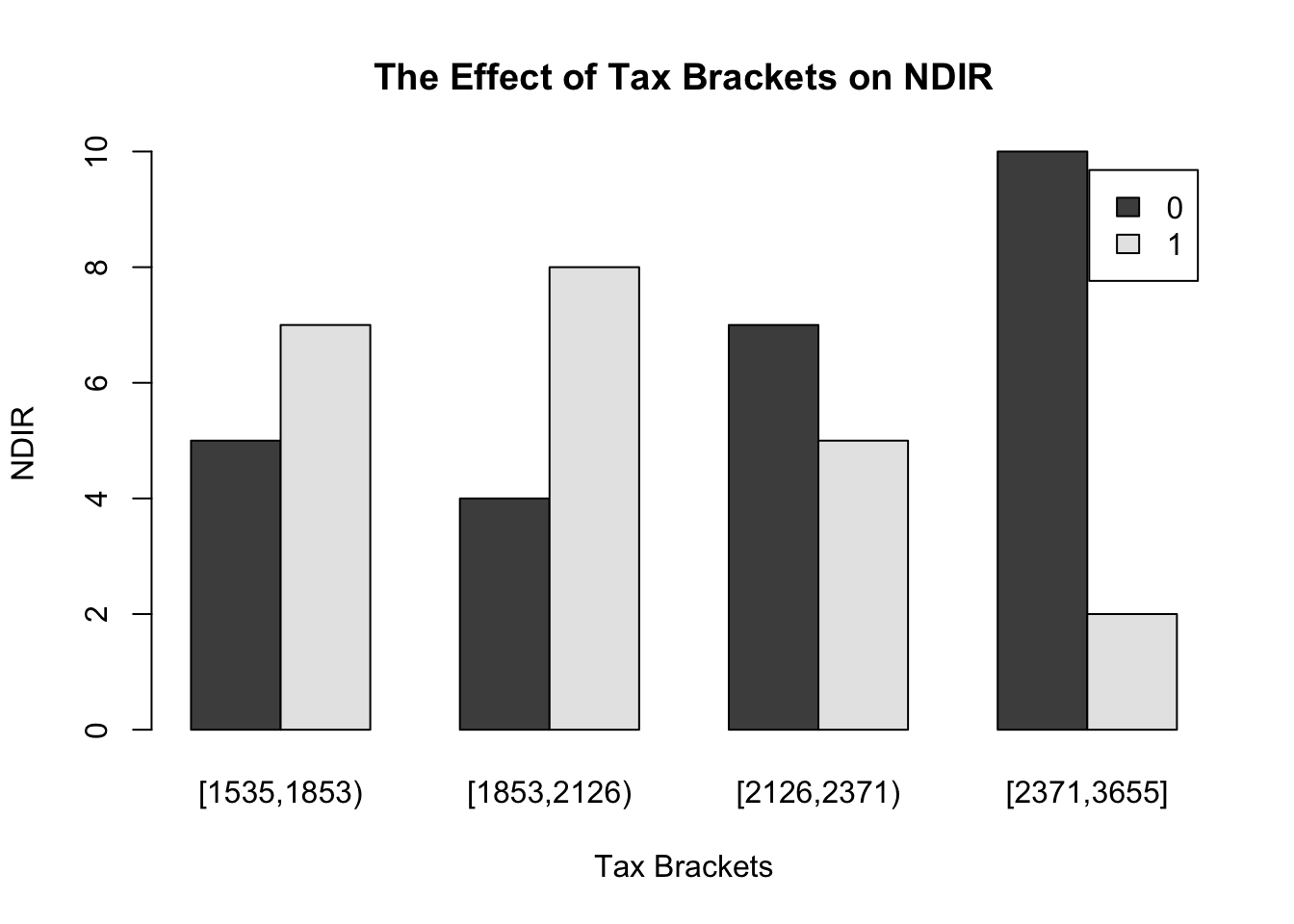
# Identifying the mean of HW4 for later usage: mean= 10.88854, click run!
mean(HW4$NDIR)

[1] 10.88854

# Creating a new dummy variable, i.e. above 1 or below 0 mean, click run!
HW4$NDIR_dummy <- ifelse(HW4$NDIR>=10.88854, 1, 0)

# Creating taxes into an ordinal variable with 4 equally sized bins, click run!
HW4$tax_ord <- cut2(HW4$Taxes, m=12)

# Creating cross tabulation, click run!
table(HW4$NDIR_dummy,HW4$tax_ord)

   
    [1535,1853) [1853,2126) [2126,2371) [2371,3655]
  0           5           4           7          10
  1           7           8           5           2

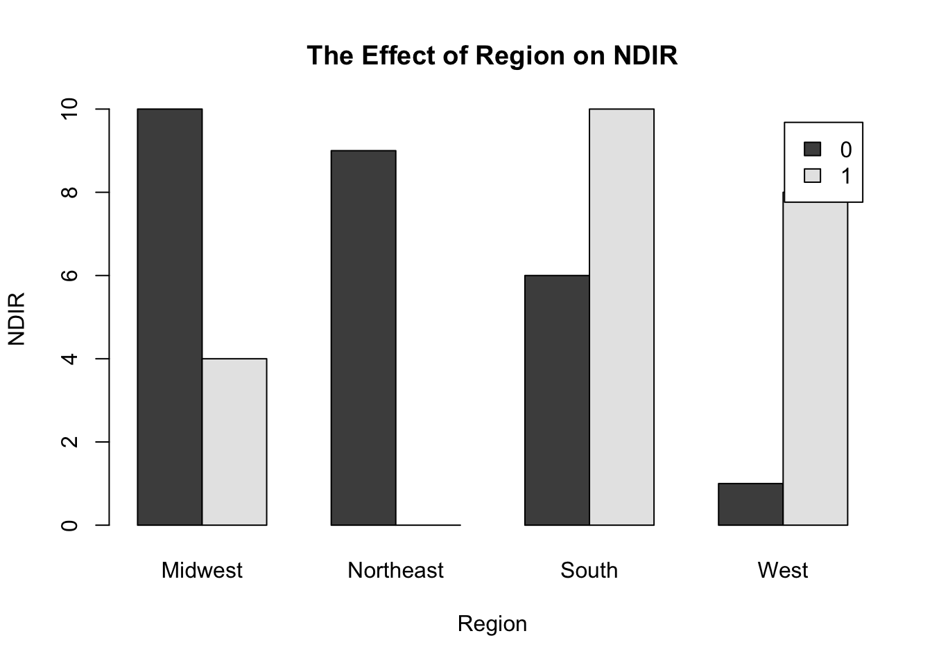
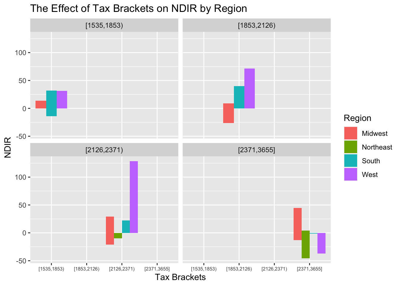
# Creating bar plot, click run!
barplot(table(HW4$NDIR_dummy,HW4$tax_ord), beside=TRUE, main= "The Effect of Tax Brackets on NDIR", xlab= "Tax Brackets", ylab= "NDIR", legend = TRUE)

barplot(table(HW4$NDIR_dummy,HW4$Region), beside=TRUE, main= "The Effect of Region on NDIR", xlab= "Region", ylab= "NDIR", legend = TRUE)

# Code for a Table with Embedded Charts
# ggplot(df,aes(z,x,fill=as.factor(y)),angle=45,size=16)+ geom_bar(position="dodge",stat="identity") +facet_wrap(~z,nrow=3)

# Creating Table with Embedded Charts, click run! 
df <- data.frame(HW4)
p <- ggplot(df,aes(tax_ord,NDIR,fill=as.factor(Region)),angle=45,size=5)+ 
  geom_bar(position="dodge",stat="identity") +facet_wrap(~tax_ord,nrow=3)
p + ggtitle("The Effect of Tax Brackets on NDIR by Region") + xlab("Tax Brackets") + ylab("NDIR") + guides(fill=guide_legend(title="Region")) + theme(axis.text.x = element_text(size = 6))